

How To Set Up A Pivot Table In Excel 2010
If you lot are in the field of finance or bookkeeping, you already know that near of the job opportunities require intermediate or advanced Excel skills. Some of the about common Excel functions in these roles are Pivot Tabular array and VLOOKUP.
This article will outline the nuts of a pivot table. Go here if you lot want to learn more than most VLOOKUP. As well, be sure to check out the alternative to VLOOKUP, a function called INDEX-Friction match.

Create a Pivot Table in Excel
What is pin tabular array? Simply put, a pin table is i of the built-in functions that you can use to quickly create a summary table based on a large set of information in Excel.
Imagine if y'all ain an online shop that sells different models of mobile phones with sales information as shown below. Download sample spreadsheet.
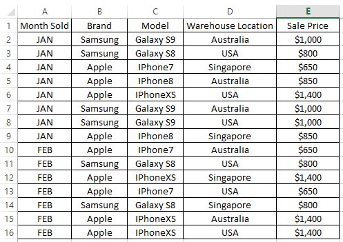
After doing business for about ii months, you are curious if you have sold more product in the first month or the second. Y'all would too like to know whether you have sold more than Apple products or Samsung products. Lastly, y'all would similar to know the total sales received in each calendar month.
The pivot table is the perfect candidate for getting a quick summary without needing to employ whatsoever Excel formula, such as count or sum. The answers to the above questions tin can be produced in a matter of seconds once y'all know how to work with a pivot table.
Here are pace-past-footstep instructions for creating a pin tabular array.
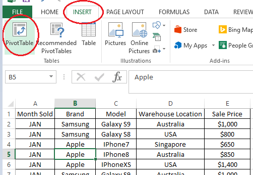
STEP ane – Create a pivot table past clicking in any of the cells within the data table, then go to the top tab in Excel and select Insert -> Pin Table .
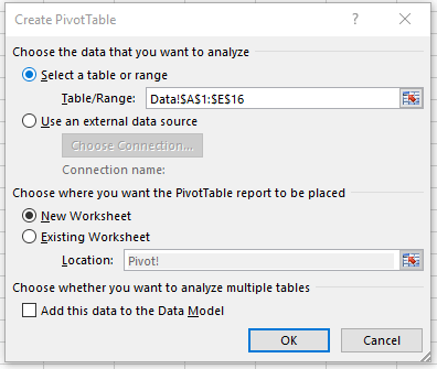
STEP 2 – A option window will appear and information technology should automatically determine the full range of the table based on the cell where you clicked earlier. For this example, we're calculation our pivot table to a new worksheet, so it'll exist easier to come across.
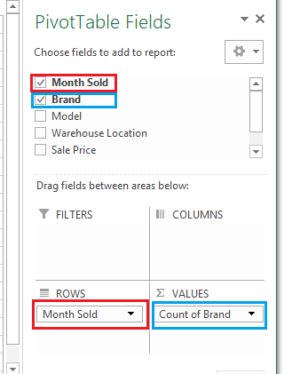
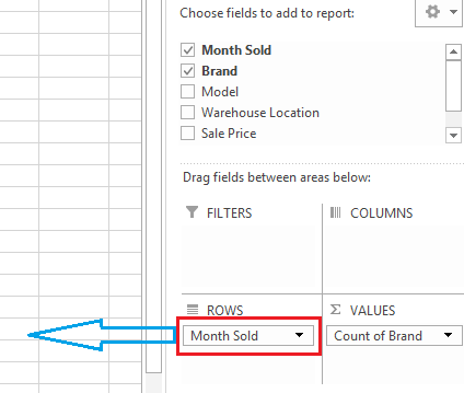
Step 3 – Click on the bare pivot table created in the new sheet. You volition observe a Pivot Table Fields volition announced on the correct side of your spreadsheet. This is where you drag-and-drop to create the quick summary.
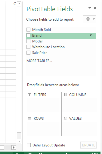
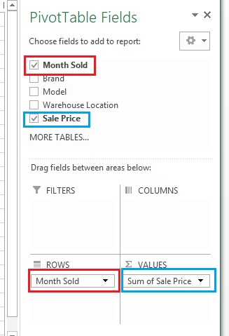
Footstep four – To know the number of mobile phone sold each month, drag Calendar month Sold to the ROWS area and Brand to VALUES area.
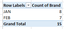
You will discover that the Pivot Table volition be automatically updated to testify the number of rows for each month, which indicates number of mobile phone sales for each month.
If you elevate Model or Warehouse Location to VALUES instead of Brand, it volition produce the same numbers for each months every bit it is but referring to the total count of rows in each Month Sold. Looks similar nosotros sold more phones in JAN compared to FEB.
STEP five – To know whether more Apple tree or Samsung products were sold in your store, you can reuse the same pivot tabular array without needing to create a new one.
To do this, you tin can clear the selection that you no longer demand (past dragging the data field out of the Expanse and dropping it anywhere on the spreadsheet).
Adjacent replace it with Make in the ROWS box.
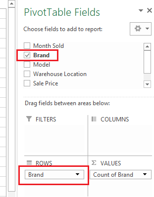
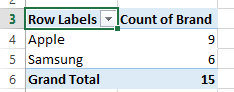
The pin tabular array will be instantly be updated to show total number of rows, grouped by Brand (i.due east. Full number of product sold by Brand to date). Yous actually sold more Apple product compared to Samsung.
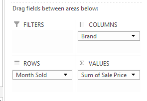
Step 5 – Lastly, to know how much yous have received in sales in each of the months, we will exist reusing the same Pivot Table.
Clear out the Brand field and drag Month Sold back to the ROWS area. Every bit we specifically desire to know the total sales, clear the VALUES area and drag in Sale Price as shown below.
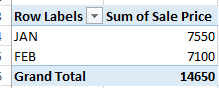
Equally the Sale Toll column in the original dataset is in number format, the pivot table will automatically sum up the Sale Toll, instead of counting the number of Sale Price rows. Voila, y'all accept received $7,550 in January and $7,100 in Feb.
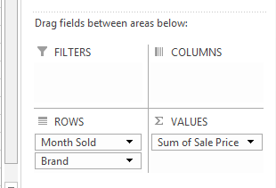
Try to play effectually and drag the fields as per below and see what is the upshot of the pivot table.
This is just scratching the surface of what pin table tin can do, but it will give you lot a proficient basic understanding to showtime with. Happy exploring!
Tips: If the Pivot Table Fields pane on the right of the spreadsheet goes missing, endeavor to hover your mouse over the pivot table, right click and choose Show Field List. That should bring it back upwards. Enjoy!
Do non share my Personal Data.

How To Set Up A Pivot Table In Excel 2010,
Source: https://helpdeskgeek.com/office-tips/how-to-create-a-simple-pivot-table-in-excel/
Posted by: leearro1941.blogspot.com
0 Response to "How To Set Up A Pivot Table In Excel 2010"
Post a Comment